Reworking the layout in Excel to import dimensions, part I
- Aug. 14, 2014
| Example files with this article: | |
Introduction
We all create dimensions in TM1, either manually (copy/paste), either through an automatic import (Turbo Integrator - TI). Recently I got an Excel file from the customer to be used for a dimension. The Excel file contained the accounts in the Balance Sheet, including their hierarchical structure. The screenshot below shows the first part of the (long) dimension:
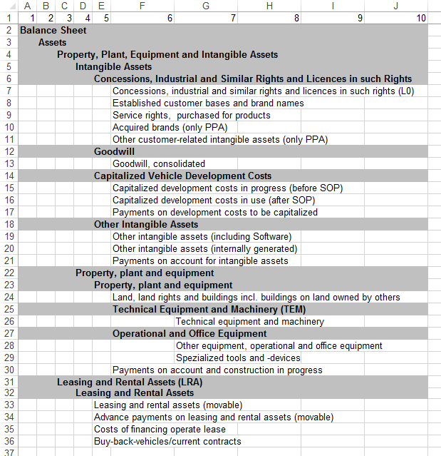
The list goes on for several hundreds of lines. How do we go about creating a TI process to set up the Balance Sheet account dimension based on this Excel file (without working a couple of hours to manually rework the layout to something that TI consumes more easily)?
-
In general, we have 2 types of input files for dimensions:
- a file always containing 2 columns: parent account and child account. Accounts in the first column can - themselves - be the parent of other accounts, and will appear several times in the list.
- a file containing a variable number of columns: from left to right (or right to left), each row in the input file consists of the hierarchical structure of a certain element. No empty cells in between.
Well, the file I received was not really either of the 2 possibilities. With extensive programming in TI, one might be able to load it, but this is not a viable solution. We would better lay out the file differently / conveniently, to limit the advanced coding needed. Not only now less coding, simple coding, also for future maintenance of the model (dimension).
Practical solution
That was what I was faced with. Without having lots of time to do this manually (and not really error proof), I decided to throw in a few Excel formulas. Yes, a few functions, not tens and tens of formulas, nested IF's, 20 helper columns, difficult lookups, … This being said, the formulas go beyond the usual SUM and IF functions. But I will explain my formulas :-) Please study the formulas, you will most likely learn new and innovative ways of using Excel functions.
-
My three step approach towards success:
- Use some formulas to get a better layout of the data
- Save the Excel file as .TXT or similar
- Write a TI process to import the Balance Sheet accounts into a dimension
Formulas
That was what I was faced with. Without having lots and lots of time to do this manually (and not really error proof), I decided to throw in a few Excel formulas. Yes, a few functions, not tens and tens of formulas, nested IF's, 10 or so hidden helper columns, difficult lookups, … This being said, the formulas go beyond the usual SUMand IF functions. But I will explain my formulas :-) Please study the formulas, you will most likely learn new and innovative ways of using Excel functions.
The goal is to rework the above layout to one where you only have 2 columns: Child account (N or C type), Parent account (C type). Here is the result:

-
Columns M and N contain the end result, column L is the only helper column. Here is the explanation of the formulas:
- column L: =MATCH("zzzzz";A2:J2;1)
As every row has 1 text value (the account name), we can use the MATCH function to search for it and return the cell position within the range A2:J2. The "zzzzz" might seem strange. We don't know what we are looking for as the text, so let's search for an alphabetically "big" text string likely "zzzzz". The search within the MATCH function stops when it hits the last textual value that is just (textually) smaller than the lookup value of "zzzzz". Hence, we stops at the only text in the row. - column M: =INDEX(A2:J2;L2)
Since we know the position of the account name, let's retrieve it with the INDEX function. So it's no magic, it's 2 easy functions that do the magic for us! - column N: =IF( L2 = 1; ""; LOOKUP("zzzzz"; INDEX($A$2:$J2; ; L2-1 )))
If the account is found at position 1, we do not a new parent and so the parent is empty (""). In all other cases, let's subtract 1 from the position (L2 - 1). Then we do a lookup - but not an easy one. See screenshot for the calculation of cell N6: =IF( L6 = 1; ""; LOOKUP("zzzzz"; INDEX($A$2:$J6; ; L6-1 )) ). We look up the word "zzzzz" in an approximate match in the range $D$2:$D6. The 6 in D6 is relative: look for the last non-empty text cell at 1 level higher up in the hierarchy (L6-1). This $D$2:$D6 is the result of the INDEX function applied to the range of all cells until the active row (6 in this case), where we "filter out" in that range (A2:J6) the 4th column (column D) since we use L6 - 1. Level 5 accounts lookup the last account name at level 4, in plain English. So we look for text in the purple range $D$2:$D6, and end up effectively in the green cell. See explanation 1 for how to return the last textual cell from a range. Here it's a column where in point 1 it was a row. Point 1 used the MATCH function, point 3 uses the LOOKUP function, since we need to return text instead of a relative position.

There you go… This is a matter of minutes, for about 1000 balance sheet accounts. Alternative formula for column N:
=IF(L3=1;"";LOOKUP(2;1/($L$2:$L3=L3-1);$M$2:$M3))
Now THIS is interesting stuff! We first check column L for being equal to the value in column L minus 1.
This returns TRUE or FALSE, for every cell. We divide 1 by the TRUE's and FALSE's, and get either a 1, either an error message (#DIV/0!) In that array of calculated results, I do a
LOOOKUP of a value of 2: the largest value just, starting at the the end of the array, will win. So the postition of the last 1 is returned. That position is
looked up row-wise in the range in column M to get the account name. What a formula trickery!
That's it, a very straightforward Excel file that we can turn into a text file and load with TI! You can't have a simpler file to work with.
Turbo Integrator
I do not want to underestimate my esteemed readers, but for the sake of completeness, here is the contents of the Metadata tab of the TI process (variables are called vChild and vParent, respectively):
##### # Wim Gielis # https://www.wimgielis.com #####cDim = 'BS_Account'; If( vParent @<> '' ); DimensionElementInsert( cDim, '', vParent, 'C'); EndIf; DimensionElementInsert( cDim, '', vChild, 'N'); DimensionElementComponentAdd( cDim, vParent, vChild, 1);
It's not over yet
Wait, there's more… The second part of this article proposes 1 (one!) formula to create the other typical structure of a file for dimensions. The Turbo Integrator code in that article is more advanced than the one discussed here, but it is fully variable and dynamic ! A must-read article in terms of Excel and TI knowledge.
Conclusion
I have demonstrated how you can allow the customer to continue using their preferred accounts layout, while still easily generating the structure for the TM1 dimension. No VBA coding, very simple TI coding, and a flexible solution towards increasing or decreasing the number of levels/hierarchies.
