Overlapping date ranges, part II
- Jul. 11, 2014
| Example files with this article: | |
Introduction
This page is the continuation of the first part, where we looked at overlapping date ranges. I introduced a practical case, namely, showing graphically the periods of June and July where:
- Students (can) face exam periods
- A major soccer tournament is organised
- The overlap between the 2 previous periods
The result was like this:

-
In the second part of the article, I will mainly do 3 things:
- explaining the formula to calculate overlapping date periods
- showing my conditional formatting rules
- demonstrating an interesting trick using data validation and conditional formatting (CF for short)
Calculating overlaps
The formula in cell P4 is as follows:
=IF(MIN(N($I4),N($J4))=0,IF(AND(date_>,=$C4,date_<,=$D4),1,0),
IF(MIN(N($C4),N($D4),N($I4),N($J4))=0,0,
IF(OR(date_<,$M4,date_>,$N4),0,
IF(AND(date_>,=$C4,date_<,=$D4,date_>,=$I4,date_<,=$J4),2,
IF(AND(date_>,=$C4,date_<,=$D4,OR(date_<,$I4,date_>,$J4)),1,3)) ) ) )
This isn't quite the easiest Excel formula that you will see today… First off, I need to tell you about that date_ component in the formula. This is in fact a formula defined with Formulas > Name Manager:
=DATE('Soccer and exams'!$A4,'Soccer and exams'!P$2,'Soccer and exams'!P$3)
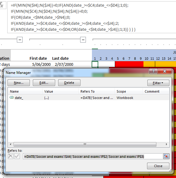
'Soccer and exams' is the sheet name, as you can see when you download the example file on top of the page. If you position the cursor in cell P4, you can use that formula to set up a "dynamic" date: it's always the date with year in column A (same row), the month always in row 3 (same column) and the day number always in row 3 (same column). The big advantage is that you can now use date_ in your cells, without typing that DATE function and its 3 input arguments over and over again, but also keep the formula shorter and easier to follow. You can use date_ in any cell of your spreadsheet, it will always refer to a year, month and day combination on the specified absolute and relative reference cells.
Going back to the formula in cell P4. In fact, all of the days in June and July (columns P to BX) for all years use the same formula because I use relative cell references. The formula returns 4 possible outcomes:
- Outcome 0: formatted without fill color - no exams and no soccer tournament
- Outcome 1: formatted in red - exams and no soccer tournament
- Outcome 2: formatted in orange - both exams and a soccer tournament
- Outcome 3: formatted in green - no exams but a soccer tournament
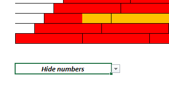
The conditional formatting (CF) to color the cells, will use the result of the formula to know how to color the cell. We will discuss the CF shortly. First, I would like to show you a nice trick that can help you greatly when setting up the file. During setup, you will want to toggle between showing the numbers (0, 1, 2, 3) and hiding these numbers. Using CF I let you do this. Cell P27 contains a dropdown where you can choose the state; showing numbers or hiding them. The CF will look at that cell, and format the cell values such that the values disappear if you choose "Hide numbers". If you choose "Show numbers" the CF rule will do nothing and the default "General" numberformatting will remain active:

The formula in cell P4 looks at the beginning dates and end dates of both periods. The formula evaluates the dates on the same row. To simplify the formula, I use 2 helper columns M and N, to track the first date of both periods, and the last date of both periods. The "current" date in the cell (June 1 to July 30 for any given year) will be evaluated with respect to the periods and their boundaries.
The N function converts the contents of a cell to a number. If the cell already contains a number, that's fine, the result is that number. If the cell contains text, the text will be converted to the number 0. Since columns I and J can contain text (a question mark) instead of dates (which are numbers in Excel), the N function can be used to always compare the input in a numeric way and to forget about the question mark. Reading the formula, we say:
- The first line in the formula returns 1 if the dates of the tournament are unknown but the date is in an exam period
- The second line in the formula returns 0 if dates are not filled in
- The third line in the formula returns 0 if the date is outside the dates of a tournament
- The fourth line in the formula returns 2 if the date is both within the exam period and the soccer tournament
- The fifth line in the formula returns 1 if the date is in an exam period but not during a tournament; if not true, then 3 is returned
Conditional formatting
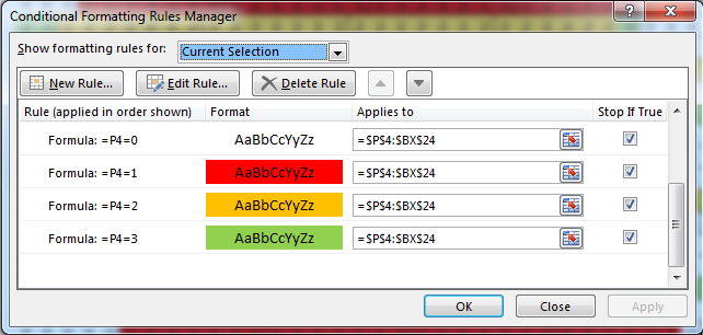
Now it is time to have a look at the CF. All CF rules apply to all 61 days (30 days for June, 31 days for July). Because I cannot resize the screen for the CF rules manager, here are the rules in 2 screenshots:

- Rule 1 instructs to have horizontal borders between rows (years).
- The objective of Rule 2 is to toggle between showing numbers in the cells, and hiding the numbers. Cfr. infra for the explanations.
- Rules 3 and 4 will apply the week border to the left of a Monday and to the right of a Sunday. The WEEKDAY function is used to see what weekday our date_ is. So yes, you can use the formula for date_ also in the conditional formatting!
- Rule 5 has the aim to format the cells when the result is 0 in the cell (no exams, no tournament). If being pedantic, you could say that this rule can be left out. In any case, unlike the previous rules, this rule has the "Stop If True" column marked: if the value is 0, upcoming rules are not treated anymore.
- Rule 6, 7 and 8 are similar, only the colour of the fill changes, depending on the numeric result in the cell (1, 2, 3). Each time, "Stop If True" is checked, because the values 0, 1, 2, 3 are mutually exclusive.
Done!
So, there you go, conditional formatting for highlighting overlapping date periods, indicating weeks as well. Hope you learnt something new with these 2 articles!
